Download: https://osdyn.ifremer.fr/pyweb/notebooks/utils/plot/heatmap.ipynb
Visualize correlation from heatmap
[1]:
import numpy as np
import os
import pandas as pd
import matplotlib.pylab as plt

from osdyn.utils.plot.heatmap import heatmap
[2]:
def corrplot(
    data,
    size_scale=500,
    marker="s",
    size_range=[0, 1],
    color_range=[-1, 1],
):
    """
    Dedicated to correlation plots but can be used for other purposes.

    Parameters
    ----------
    data : pandas.Dataframe
        data containing the x axes, y axes, values.
    size_scale : int, optional
        multiplicator of data value. The default is 500.
    marker : str, optional
        "s" "c" "t"... The default is "s".
    size_range : list of 2 int or float, optional
        Values to anchor the sizes. The default is [0, 1].
    color_range : list of 2 int or float, optional
        Values to anchor the color. The default is [-1, 1].

    Returns
    -------
    Call heatmap

    """
    corr = pd.melt(data.reset_index(), id_vars="index").replace(np.nan, 0)
    corr.columns = ["x", "y", "value"]
    heatmap(
        corr["x"],
        corr["y"],
        color=corr["value"],
        color_range=color_range,
        palette=plt.get_cmap("seismic_r", lut=256),
        size=corr["value"].abs(),
        size_range=size_range,
        marker=marker,
        x_ticklabel=data.columns,
        y_ticklabel=data.columns[::-1],
        size_scale=size_scale,
    )
[3]:
# Load the Automobile dataset.
# This gets a cleaned version of UCI dataset
# found at http://archive.ics.uci.edu/ml/datasets/automobile
#data = pd.read_csv("https://raw.githubusercontent.com/drazenz/heatmap/master/autos.clean.csv")
data = pd.read_csv(os.path.join(os.environ["INPUT_DATA_PATH"],"autos.clean.csv"))
[4]:
data.corr()
[4]:
| symboling | normalized-losses | wheel-base | length | width | height | curb-weight | engine-size | bore | stroke | compression-ratio | horsepower | peak-rpm | city-mpg | highway-mpg | price | |
|---|---|---|---|---|---|---|---|---|---|---|---|---|---|---|---|---|
| symboling | 1.000000 | 0.466264 | -0.535987 | -0.365404 | -0.242423 | -0.550160 | -0.233118 | -0.110581 | -0.140019 | -0.008153 | -0.182196 | 0.075819 | 0.279740 | -0.035527 | 0.036233 | -0.082391 |
| normalized-losses | 0.466264 | 1.000000 | -0.056661 | 0.019424 | 0.086802 | -0.373737 | 0.099404 | 0.112360 | -0.029862 | 0.055045 | -0.114713 | 0.217299 | 0.239543 | -0.225016 | -0.181877 | 0.133999 |
| wheel-base | -0.535987 | -0.056661 | 1.000000 | 0.876024 | 0.814507 | 0.590742 | 0.782097 | 0.572027 | 0.493244 | 0.158018 | 0.250313 | 0.371147 | -0.360305 | -0.470606 | -0.543304 | 0.584642 |
| length | -0.365404 | 0.019424 | 0.876024 | 1.000000 | 0.857170 | 0.492063 | 0.880665 | 0.685025 | 0.608971 | 0.123952 | 0.159733 | 0.579821 | -0.285970 | -0.665192 | -0.698142 | 0.690628 |
| width | -0.242423 | 0.086802 | 0.814507 | 0.857170 | 1.000000 | 0.306002 | 0.866201 | 0.729436 | 0.544885 | 0.188822 | 0.189867 | 0.615077 | -0.245800 | -0.633531 | -0.680635 | 0.751265 |
| height | -0.550160 | -0.373737 | 0.590742 | 0.492063 | 0.306002 | 1.000000 | 0.307581 | 0.074694 | 0.180449 | -0.060663 | 0.259737 | -0.087027 | -0.309974 | -0.049800 | -0.104812 | 0.135486 |
| curb-weight | -0.233118 | 0.099404 | 0.782097 | 0.880665 | 0.866201 | 0.307581 | 1.000000 | 0.849072 | 0.644060 | 0.167438 | 0.156433 | 0.757976 | -0.279361 | -0.749543 | -0.794889 | 0.834415 |
| engine-size | -0.110581 | 0.112360 | 0.572027 | 0.685025 | 0.729436 | 0.074694 | 0.849072 | 1.000000 | 0.572609 | 0.205928 | 0.028889 | 0.822676 | -0.256733 | -0.650546 | -0.679571 | 0.872335 |
| bore | -0.140019 | -0.029862 | 0.493244 | 0.608971 | 0.544885 | 0.180449 | 0.644060 | 0.572609 | 1.000000 | -0.055390 | 0.001263 | 0.566936 | -0.267392 | -0.582027 | -0.591309 | 0.543155 |
| stroke | -0.008153 | 0.055045 | 0.158018 | 0.123952 | 0.188822 | -0.060663 | 0.167438 | 0.205928 | -0.055390 | 1.000000 | 0.187871 | 0.098267 | -0.063561 | -0.033956 | -0.034636 | 0.082269 |
| compression-ratio | -0.182196 | -0.114713 | 0.250313 | 0.159733 | 0.189867 | 0.259737 | 0.156433 | 0.028889 | 0.001263 | 0.187871 | 1.000000 | -0.214514 | -0.435780 | 0.331425 | 0.268465 | 0.071107 |
| horsepower | 0.075819 | 0.217299 | 0.371147 | 0.579821 | 0.615077 | -0.087027 | 0.757976 | 0.822676 | 0.566936 | 0.098267 | -0.214514 | 1.000000 | 0.107885 | -0.822214 | -0.804575 | 0.809575 |
| peak-rpm | 0.279740 | 0.239543 | -0.360305 | -0.285970 | -0.245800 | -0.309974 | -0.279361 | -0.256733 | -0.267392 | -0.063561 | -0.435780 | 0.107885 | 1.000000 | -0.115413 | -0.058598 | -0.101616 |
| city-mpg | -0.035527 | -0.225016 | -0.470606 | -0.665192 | -0.633531 | -0.049800 | -0.749543 | -0.650546 | -0.582027 | -0.033956 | 0.331425 | -0.822214 | -0.115413 | 1.000000 | 0.972044 | -0.686571 |
| highway-mpg | 0.036233 | -0.181877 | -0.543304 | -0.698142 | -0.680635 | -0.104812 | -0.794889 | -0.679571 | -0.591309 | -0.034636 | 0.268465 | -0.804575 | -0.058598 | 0.972044 | 1.000000 | -0.704692 |
| price | -0.082391 | 0.133999 | 0.584642 | 0.690628 | 0.751265 | 0.135486 | 0.834415 | 0.872335 | 0.543155 | 0.082269 | 0.071107 | 0.809575 | -0.101616 | -0.686571 | -0.704692 | 1.000000 |
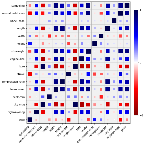
[5]:
plt.figure(figsize=(8, 8))
corrplot(data.corr(), size_scale=300)